We would like to thank the Nebraska Corn Board for funding this study and making this internship position possible at the University of Nebraska-Lincoln.
1. Introduction
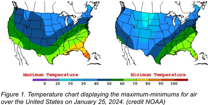
Midwesterners are no strangers to fog. In January of 2024, nearly a third of the United States found itself blanketed in fog. The major portion of this event occurred over the Midwest. It didn’t just make for blustery weather; it led to numerous flight delays, vehicle accidents, and loss of life (Livingston). Three days in a row, this event broke records for how many counties were placed under dense fog advisory by the National Weather Service. Moist air blown in from the Gulf of Mexico had settled over the winter landscape (see figure one). To note, the United States also experienced heavy snowfall before this. The high amount of snow cover was crucial to allowing the formation of advection fog. While the immediate cause is understood, we have less knowledge of the repercussions this had on the atmosphere. Key Point: Exploring potential relationships between winter fog and subsequent summer rain is vital for future research and can improve forecasting abilities.
- Fog As Weather
Fog is typically viewed as a paired event with other atmospheric phenomena. Chiefly, it is treated as a product of precipitation, with many papers seeing it form during or directly after precipitation events. It is within that action-reaction relationship fog has been generally measured. Furthermore, fog is studied as a dimension of multiple different frameworks, from human health to its impacts on the transportation sector. It is seldom viewed as a singular event, and even rarer is it treated as a precursor event.
To that end, fog is internationally defined as a loss of visibility below 1 kilometer (Glickman 2000). Further sub-definitions relate to differentiating between fog, haze, and mist for aviation forecasting. To best suit our purposes, we address fog as a whole concept. This definition is wide enough to include pollution-based fogs and account for different fog droplet composition types. Beyond the visual definition, a meteorological standard for researchers to use is defined by the individual study. There are advantages to the World Meteorological Organization’s broad definition, allowing regional studies to account for unique externalities that may not exist elsewhere. However, this presents problems with standardization and model bias.
Fog being treated as a product of other weather events does allow for a large amount of data. For example, it gives us data indicating optimal conditions for fog formation. Even when selecting for stricter definitions of fog, datasets will generally marry it to other factors, be it precipitation, pollution, mesospheric activity, or ground cover. Studies focused solely on identifying fog itself usually do so through remote sensing and deep machine learning. Only one of these studies identified fog as a precursor in a seeder-feeder interaction between fog and subsequent precipitation (Barros and Duan 2017). Even when doing so, it was done in the context of geography. Key Point: The current direction of a majority fog research views fog as secondary to some other system, not as a potential trigger for other phenomena.
3. Current Understanding of Fog
Working within the international definition of fog, several studies have identified commonalities when it comes to meteorological conditions for fog formation. Collating these findings allows us to form a definition that does not rely solely on observational reports or high-powered computing. Progress has been made in this direction, with a study in South Africa putting together a reference resource for airport forecasters. While their decision tree does include visual conditions, measurable with ceilometers, it also relies on wind speed and temperatures. Additionally, the researchers recommended moving away from the recording of ‘fog days’ to instead class these instances as ‘fog events’ for the sake of accuracy (Dyson et al 2013).
When studying conditions prior to a fog event, a twenty year examination of New York City and the surrounding region placed high significance on temperature. Namely, the presence of an inversion close to the ground (Tardif and Rasmussen 2007). While the study was performed over a coastal region, it still provides a significant finding when it comes to atmospheric mixing.
In terms of geography similar to the Midwestern United States, a thirty year study of the Pannonian Plains in Serbia found relationships between both time of year and wind speed. They reported that fog event occurrence peaked in October, during the seasonal shift between fall and winter. Furthermore, 71% of their fog events occurred with little to no wind in the area and a notable absence of cloud cover (Vujović and Veljović 2019). These fog events were radiation fog. They acknowledged a weakness in their methodology, primarily relying on visual observations. The study made recommendations for replicating their methods but with satellite imagery at some point in the future.
Isolating fog from precipitation-specific conditions allows us to find overarching patterns in local climatologies closer to home. A study of Northern Utah’s ASOS recordings over a decade found that weaker synoptic systems preceded a fog event, usually with a ridge moving from the West (Hodges and Pu 2015). It should be noted that the Eastern topography of Utah is a mountain range.
Within the North American Great Plains, studies have been done to try and identify synoptic conditions optimal for fog events. Of the ten categories defined in a twenty five year study by the University of Illinois, they found a total of 26% of fog events occurred under a high pressure system. Low pressure systems were credited with 15% of fog events when no fronts were observed in the area. They also identified a positive relationship between fog size and its duration, the bigger a fog bank the longer it lasted (Westcott 2004).
A further study by the University of Illinois confirmed the relationship between fog size and duration. Further, they found that the best predictor for a fog event’s duration in the Midwestern United States appears to be “fog onset time and the physical dimensions of the fog event…” (Westcott 2005). The closer to midnight a fog event occurs, the longer its duration. An additional finding of note was an apparent range of wind speeds relating to fog event duration (see figure 2).

Of highest interest for our purposes, two studies give us a strong foundation for investigating interactions between fog events and subsequent precipitation events. A study regarding Canadian temperature-precipitation trends found additional links between temperature changes and events. Of their findings, 90% of reported fog events were followed by precipitation. These findings were measured across all of Canada, in climatology datasets ranging from 7 years long to 55 years long. It should be noted that those precipitation events made up 50% of their findings across the study’s multiple datasets (Isaac and Stuart 1991).
Specifically mentioning the relationship between fog and precipitation is a ten year study performed over the Southern Appalachian Mountains. Using both ASOS and satellite data, researchers identified a seeder-feeder interaction between fog and low level clouds that was found to increase precipitation intensity by ten-fold (Barros and Duan 2017). Key Point: Evidence exists that a trend may be indicated between fog and resulting rain, though it could be influenced by topography.
4. The Use of Satellite Imaging Systems
Multiple studies have made mention or taken advantage of the potential of satellite imaging. Remote sensing can be incredibly effective for sole fog observations and fog-precipitation interactions. It is not always possible for on the ground recording of weather events due to lack of station availability, lack of proper instrumentation on stations, or even different data-recording standards between organizations. Remote sensing giving a ‘birds eye’ view of weather events allows non-local researchers to observe and measure phenomena for their own experimentation. Of the three studies relevant to our purposes, accuracy in identification is promising but variable with yearly seasons. One study eliminated the inefficiencies in their identification scheme by pairing their data with ASOS ceilometers. These studies can be costly in terms of resources and computation.
One benefit is seen in using thermal imaging cameras on satellites to solely identify fog and low level clouds. A ten year study of European satellite data, where researchers reviewed images taken during times ground stations reported fog, found that satellite imaging can have up to 93% accuracy. Unfortunately, this high accuracy rate only lasted for winter months and dropped dramatically to 38% during the summer (Egli et al 2017). One problem identified with this study was that in datasets lacking records of the base height of cloud cover, it was significantly harder for fog to be identified by satellite.
There have been promising attempts to automate satellite identification of fog events. Research in China took a two year dataset of 3122 fog event images and trained a deep learning algorithm to identify them. By the end of the study, the algorithm had 84% accuracy (Ran et al 2022). It should be noted these images were specifically taken during dawn and dusk hours, not any other time. Key Point: The use of remote sensing for researching fog has utility, but is costly for scientists to integrate into their studies.
5. Defining Fog without Observation or Satellite
Not every dataset available to researchers may come with visual observations to definitely say a fog event occurred. In the interest of precision, a ‘blind’ meteorological definition accounting for multiple instruments should be established. In the interest of precision, we established a ‘blind’ meteorological definition accounting for multiple instruments. For the sake of breadth, we did not factor formation types into these metrics. These metrics normalized readings across multiple scientific studies on fog and averaging for simplicity:
- Wind Speed - 5 m/s or lower
- Relative Humidity - 90% or greater
- Temperature - Difference between temperature and dewpoint should be 2.2°C or lower
- Given the variable nature of fog event occurrence, temperature alone is not an accurate indicator. Rather, it is a relationship between temperature and dewpoint that indicates .
- Visibility - 1 km or less
6. Methodology and Data
We accessed historical METARs from seven ASOS stations across Nebraska using archived data from the Iowa Environmental Mesonet for the period between 1964-2024. Using Python code, we filtered the records through our ‘blind fog’ definition and compiled them into one sequence. Then, we compiled precipitation records for both the 24 hours after each fog event and the total amount of precipitation accumulated across each year’s summer months, defined as June, July, and August (JJA). We then accumulated the total fog events by winter season, defined as December, January, and February (DJF). In summary, both fog and precipitation records were compiled into a ‘24 hour’ sequence and a ‘seasonal’ sequence.
We also compiled Oceanic Nino Index (ONI) data from the National Oceanic and Atmospheric Administration (NOAA) to determine if there was a relationship between the phase of the El Nino Southern Oscillation (ENSO) and fog days and subsequent summer precipitation. The ONI is used to determine whether there was an El Nino (positive ONI), a La Nina (negative ONI), or neutral conditions (index around 0) and the magnitude of El Nino and La Nina.

7. Results and Discussion
A Chi-Square of Independence test for each of the seven stations’ 24 hour sequence indicated across the board that there is a relationship between fog and rain; however, a follow up Phi coefficient test showed the relationship is weak at all sites. Correlation and covariance testing of seasonal totals also confirmed these findings (see figure four). This indicates to us that fog is not a predictor of subsequent rain . Rather, these two forms of precipitation appear to act in concert when broader atmospheric conditions that allow for higher moisture levels in the lower part of the atmosphere.

To explore this further, we plotted the seasonal sequence with the magnitude of ENSO. Linear regression of the seasonal sequence when put into this framing shows a slight positive relationship between El Niño years and high rates of winter fog and summer rain within Nebraska (see figure three). Notably, the stronger the magnitude of the El Niño the higher rates of winter fog are seen. The effect of ENSO on subsequent summer precipitation is less, though still is an overall positive correlation (see figure five). Furthermore, our results show that a higher number of winter fog days were rarely associated with much below average precipitation the following summer. The results are not conclusive enough to show that drought will be avoided in a summer after more winter fog. But it does suggest that a summer drought after an abnormal amount of winter fog is a lower probability event, especially if associated with an El Nino. Key Point: While winter fog does not directly increase chances of summer rain, Nebraska can expect to see both increased fog and rain events during El Niño years.

8. Acknowledgements
This study was funded through an Innovation & Stewardship grant by the Nebraska Corn Board.
9. References
Livingston, Ian. “Why thick fog is blanketing a record stretch of the U.S.” The Washington Post, 25 January 2024, https://www.washingtonpost.com/weather/2024/01/25/record-fog-united-states-explained/. Accessed 30 May 2025
Glickman, Todd. “fog - Glossary of Meteorology.” Glossary of Meteorology, 30 March 2024, https://glossary.ametsoc.org/wiki/Fog. Accessed 27 May 2025
Barros, Ana P., and Yajuan Duan. “Understanding How Low-Level Clouds and Fog Modify the Diurnal Cycle of Orographic Precipitation Using In Situ and Satellite Observations.” Remote Sensing, vol. 9, no. 9, 2017, p. 920. https://doi.org/10.3390/rs9090920.
Liesl L. Dyson, van Schalkwyk, and Lynette. “Climatological Characteristics of Fog at Cape Town International Airport.” Weather and Forecasting, vol. X, no. 1, 2013, pp. 1-16.
Tardif, Robert, and Roy M. Rasmussen. vol. 47, no. 6, 2007, pp. 1681–1703. https://doi.org/10.1175/2007JAMC1734.1.
Vujović, D., and K. Veljović. “Climatology of fog occurrence over a wide flat area in Serbia based on visibility observations.” International Journal of Climatology, vol. 39, no. 3, 2019, pp. 1331-1344. https://doi.org/10.1002/joc.5883.
Westcott, Nancy. “Some Aspects of Dense Fog in the Midwestern United States.” American Meteorological Society, vol. X, no. X, 2005, pp. 457-465. https://doi.org/10.1175/WAF990.1.
Westcott, Nancy. “Synoptic Conditions Associated with Dense Fog in the Midwest.” Illinois State Water Survey, vol. X, no. X, 2004, 2.4. https://www.isws.illinois.edu/.
Isaac, G.A., and R.A. Stuart. “Temperature-Precipitation Relationships for Canadian Stations.” Journal of Climate, vol. 5, no. 8, 1991, pp. 822-830. https://doi.org/10.1175/1520-0442(1992)005<0822:TRFCS>2.0.CO;2.
Egli et al. “A 10 year fog and low stratus climatology for Europe based on Meteosat Second Generation data.” Quarterly Journal of the Royal Meteorological Society, vol. 143, no. 1, 2017, pp. 530-541. https://doi.org/10.1002/qj.2941.
Ran et al. “Satellite Fog Detection at Dawn and Dusk Based on the Deep Learning Algorithm under Terrain-Restriction.” Remote Sensing, vol. 14, no. 17, 2022, p. 4328. https://doi.org/10.3390/rs14174328.